Neural Radiance Fields
By Kourosh Salahi · CS180 / 280A
This project implements NeRF completely from scratch: camera calibration, pose estimation, ray sampling, neural fields, volume rendering, and training NeRFs on both the classic Lego dataset and my own captured data. This page contains animations
Part 0 — Camera Calibration & Dataset Capture
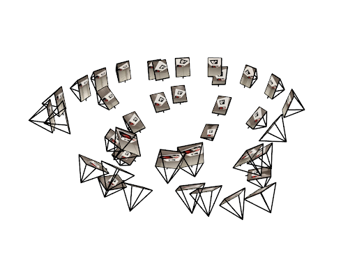
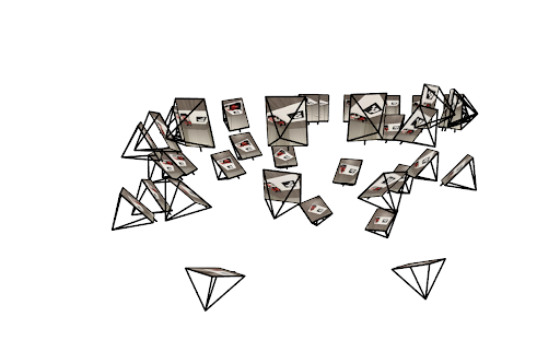
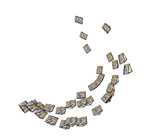
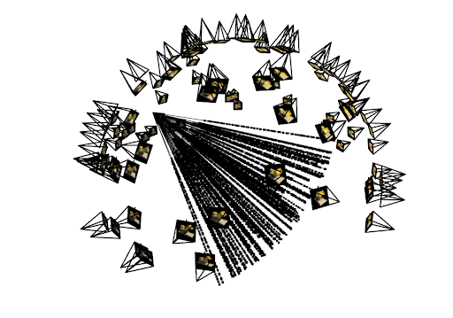
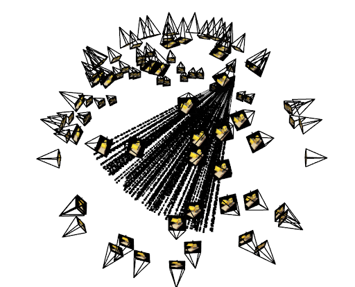
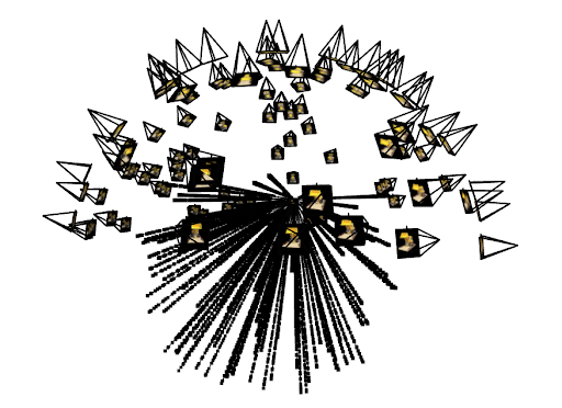
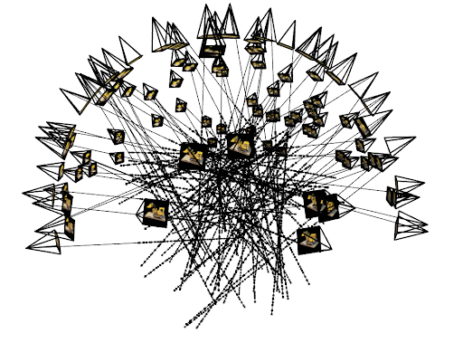
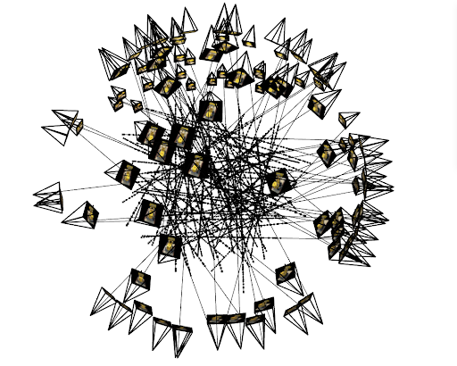
Camera Frustums Visualization
After calibrating my camera through a grid of aruco tags, and taking multiple photos of my object from different views, I was able to estimate camera poses, as visualized below.
Calibration Visualization
Part 1 — Neural Field Fitting (2D)
Model Architecture
For image fitting, I used a fully-connected network with width 256 and
positional encoding L = 10. The model takes the 2D coordinates
(after PE, dimension 4L + 2) and passes them through three
hidden layers:
- Input:
4L + 2-dim positional-encoded coordinates - Hidden layers: 3 × (Linear → ReLU), each of width 256
- Output layer: Linear → Sigmoid (predicts RGB in [0,1])
Training used Adam with learning rate 1e-2 and MSE loss.
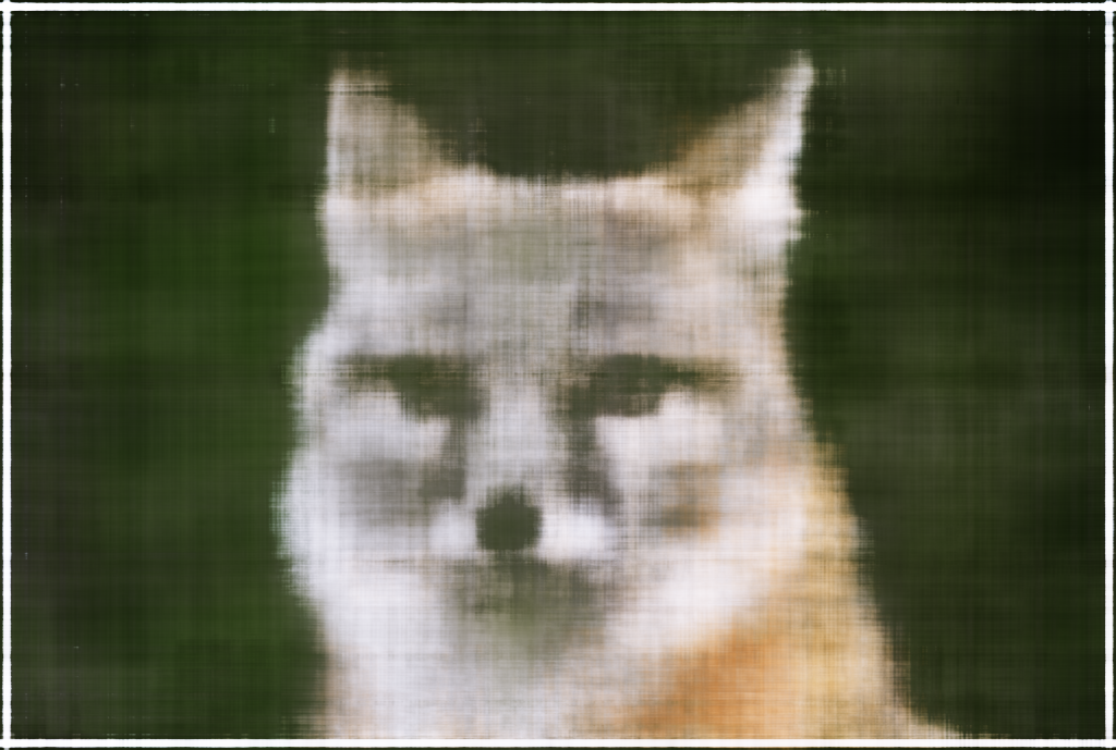
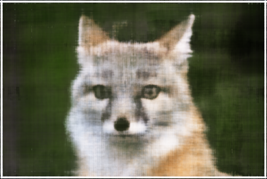
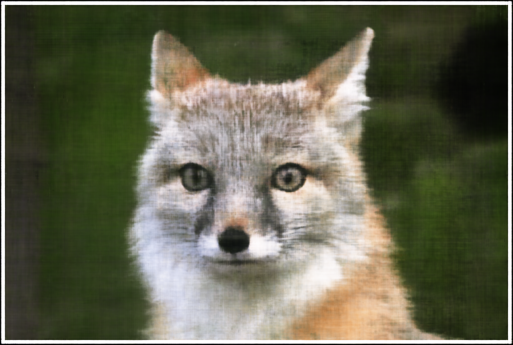
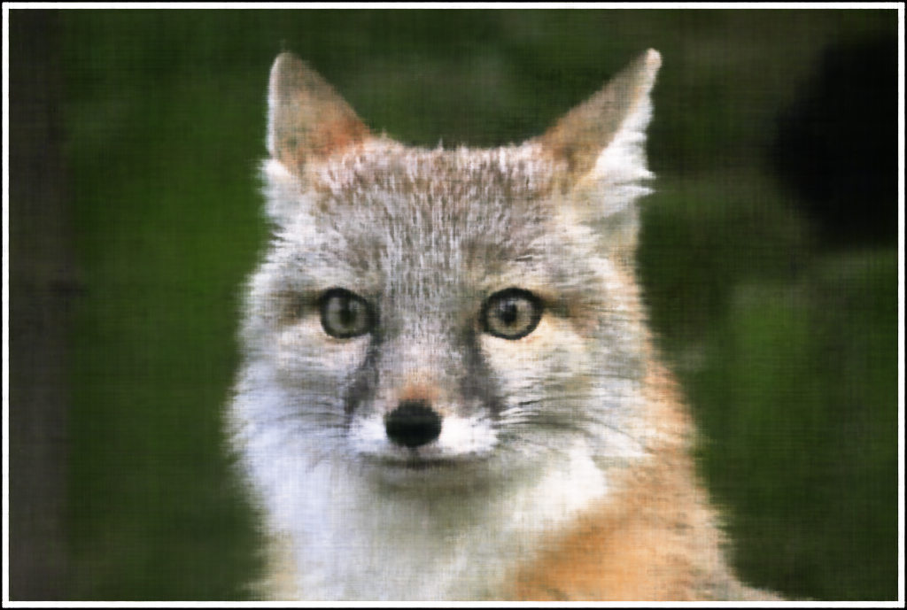
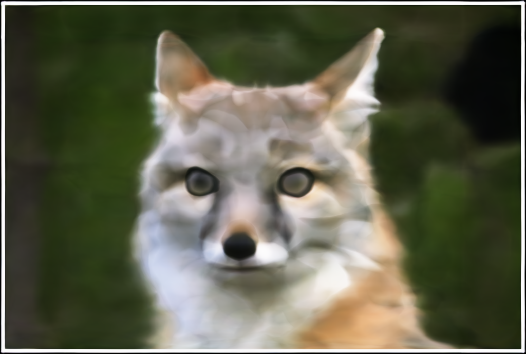
Training Progression — Fox (Width=256, L=10)
Training iterations shown: 0 → 50 → 100 → 200 → 500 → 1000 → 1999.
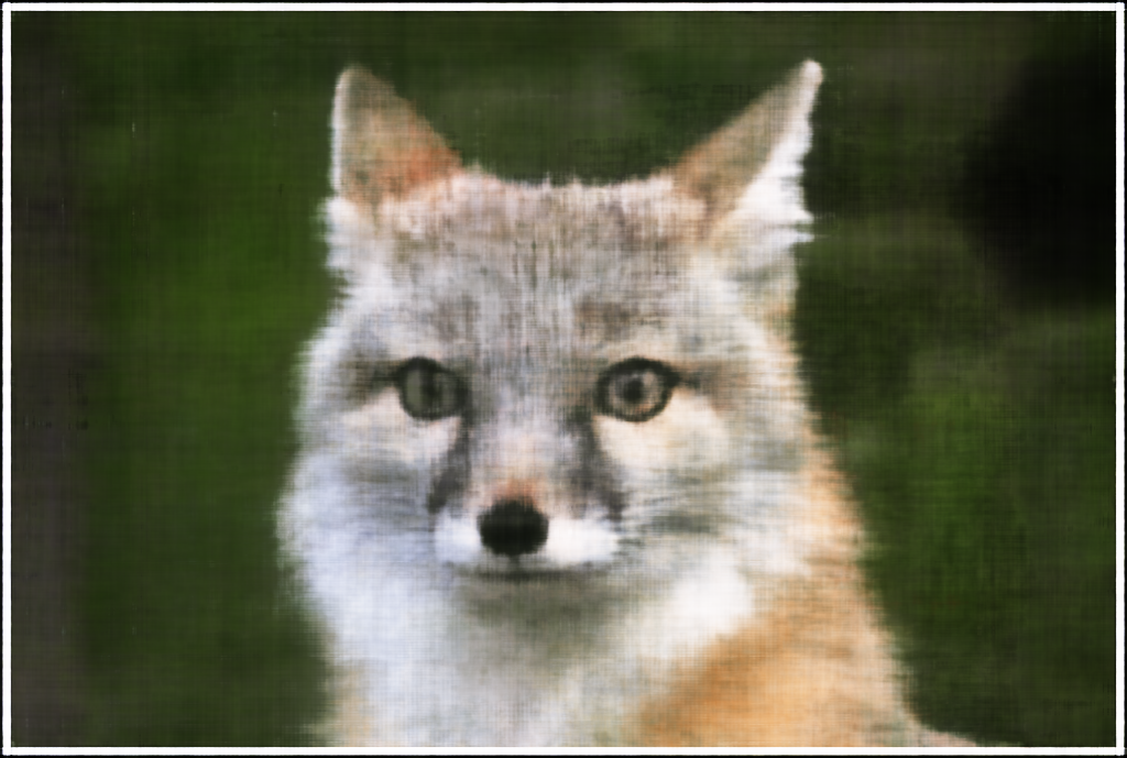
Final Results
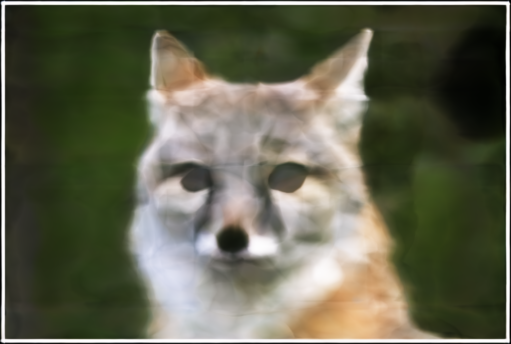
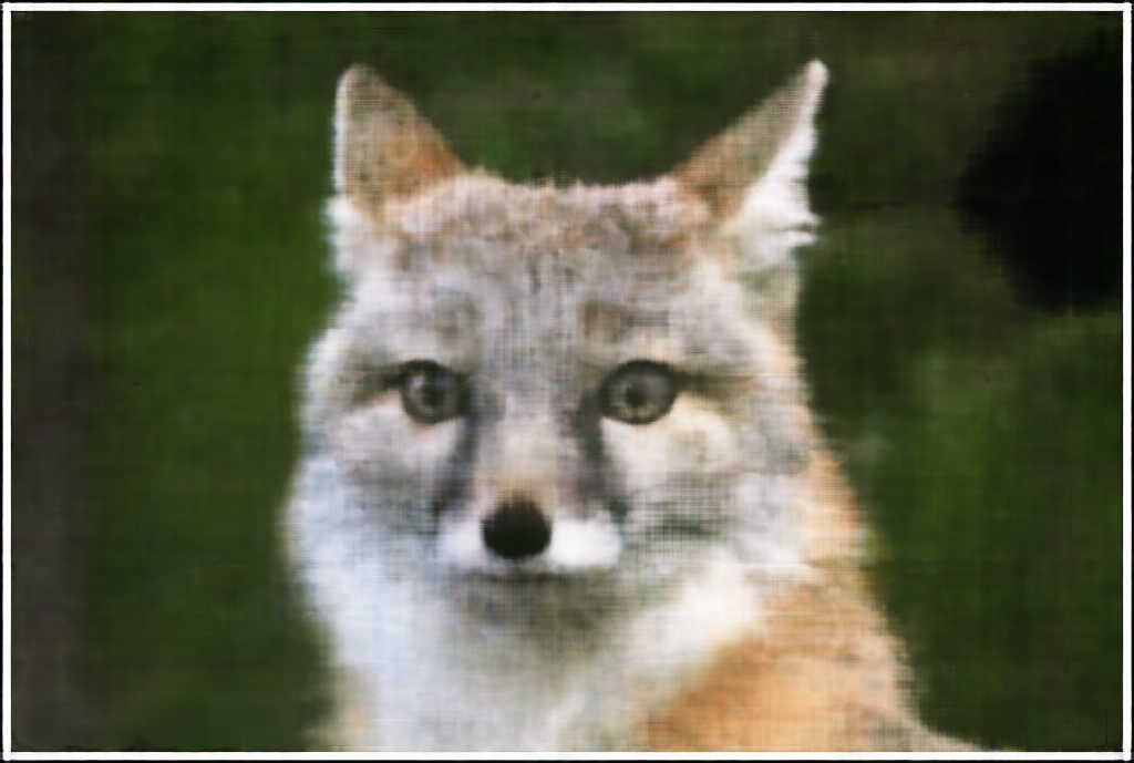
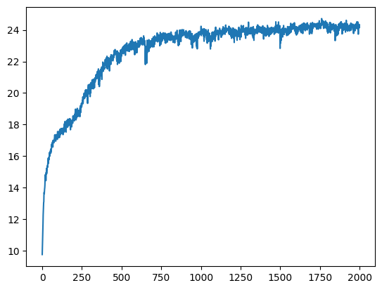
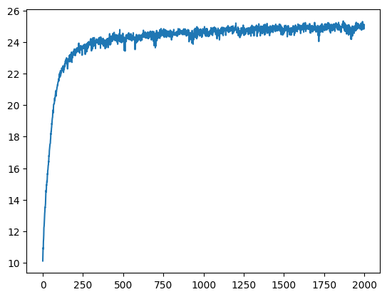
Four combinations of PE frequency (L ∈ {4,10}) and width (W ∈ {64,256}), all at iter1999. It seems as though Positional encoding has the highest effect on our overall image ouput quality.
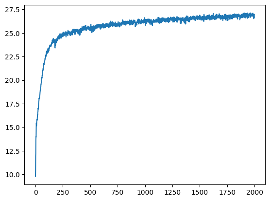
PSNR Curves (Fox)

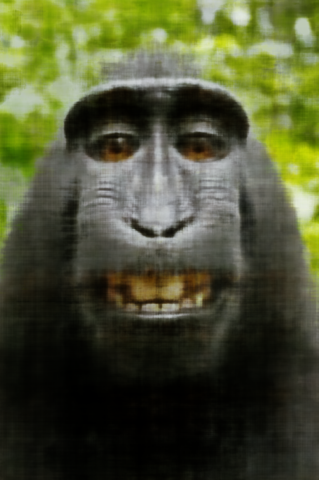
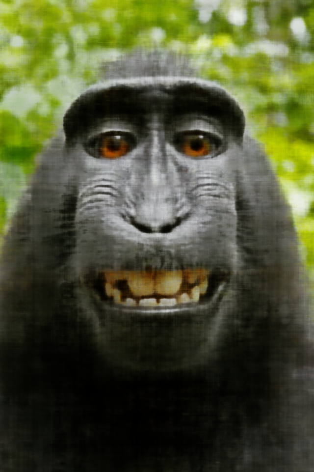
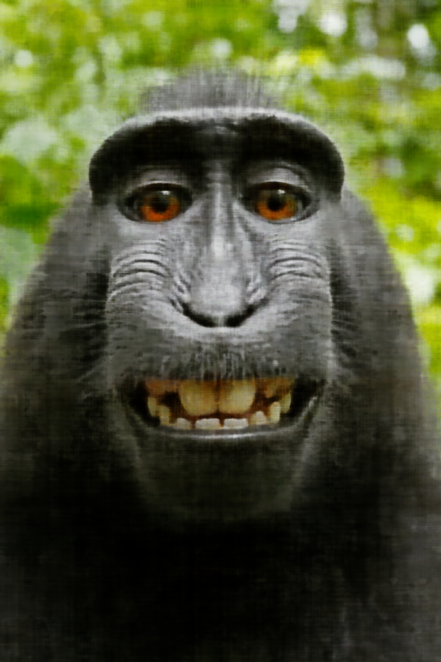
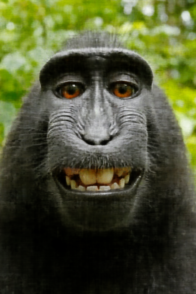
Training Progression — Monkey (Width=256, L=10)
Training iterations shown: 0 → 50 → 100 → 200 → 500 → 1000 → 1999.
Part 2 — Neural Radiance Field on Multi-View Lego
In this section, I implemented a complete NeRF pipeline: converting image pixels to 3D world-space rays, sampling points along those rays, evaluating a radiance field network, and performing differentiable volume rendering to optimize the model against multiple posed RGB images.
2.1 Camera → Ray Pipeline
-
pixel_to_camera(K, uv):
I convert pixel coordinates to camera coordinates by analytically inverting
the pinhole intrinsics. For each pixel
(u, v), I compute:(x, y, z) = ((u - ox)/fx, (v - oy)/fy, 1). -
transform(c2w, x_c):
My world-space transform builds homogeneous coordinates explicitly.
Given
x_c ∈ ℝN×3, I append a column of ones, reshape to(N, 4, 1), then left-multiply by the camera-to-world matrix:
The result is squeezed back toc2w @ [x, y, z, 1]^T → [X, Y, Z, 1]^T(N, 3). This implementation matches the mathematical camera transform exactly and is fully vectorized across all points. -
pixel_to_ray(K, c2w, uv):
After converting pixel locations to camera coordinates and transforming them
into world space, (using the previous two functions) I compute:
ray_o = c2w[:3, 3]as the origin would simply be the translation of the camera to world frame, andray_d = normalize(x_w − ray_o), as the ray direction would be the difference between our world point and the position of the camera in the world frame. This yields the origin and direction of each ray used during training.
Together, these steps implement the full pixel → camera → world → ray pipeline required for NeRF training.
2.2 Sampling Rays & Points
I use global ray sampling, where all pixels from all training images are flattened into a single pool. Each pixel is recorded with a +0.5 offset so that sampling occurs at the pixel center. At every iteration, I randomly choose N pixel indices, giving uniformly distributed rays across all views.
For each selected pixel, I compute its ray origin and direction from the previous pixel_to_ray method. Each ray is then discretized into n_samples = 64 points
between near = 2.0 and far = 6.0 using:
x = r_o + r_d · t
During training I ensure that
every portion of the ray is eventually sampled and prevent the network from overfitting to
fixed depths by adding random noise within each interval (i.e., ti ← ti + ε·Δt).
This ensures that over training, every part of the ray contributes to the reconstruction. The values n_samples, near, and far are
parameters in my implementation, and I later change them for different scenes (e.g., my real
dataset uses a smaller range), since the optimal sampling bounds depend heavily on object scale
and the physical capture setup.
2.3 Dataloader + Precomputation + Viser Visualizations
To accelerate training, I built a preprocessing stage that:
- enumerates every pixel in every image with a +0.5 center offset,
- stores their RGB values,
- stores a repeated copy of the camera extrinsic for each pixel,
- precomputes world-space
ray_oandray_dfor the entire dataset.
The dataloader then samples rays by simply indexing into these large flattened arrays. I validated correctness of UV alignment, ray orientation, and frustum consistency using Viser visualizations.
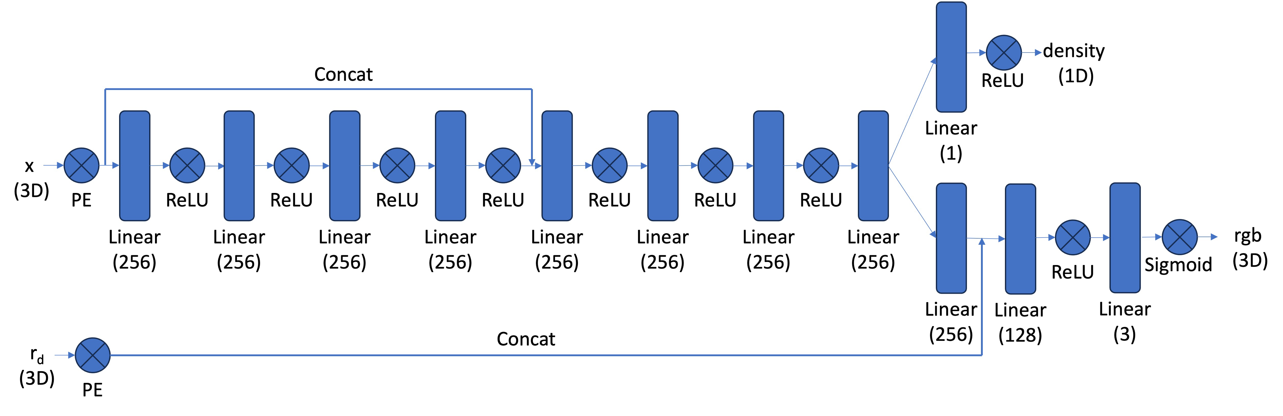
2.4 Neural Radiance Field MLP
My NeRF model closely follows the original architecture: a deep point MLP with a skip connection, a density head, and a separate view-dependent color head. Both 3D sample locations and ray directions use sinusoidal positional encoding before being fed into the network.
-
Positional Encoding:
For my implementation, 3D points are encoded using
Lx=10, giving3 + 6L = 63channels. Ray directions useLr=4, producing3 + 6L = 27channels. -
Point MLP (σ + features):
The encoded 3D point is processed by an 8-layer MLP with width 256.
At the 4th hidden layer (index 3), I concatenate the original positional encoding
back into the network, exactly matching:
Linear(256 + input_dim_x → 256). This skip connection helps preserve high-frequency spatial detail. -
Density Head (σ):
After the final point-layer, a
256 → 1linear projection followed by ReLU produces the volume densityσ. -
Color Head (rgb):
The point-MLP output is first transformed into a 256-D feature vector.
This feature is concatenated with the encoded ray direction (27-D) and passed through:
(256 + input_dim_r) → 128with ReLU,128 → 3with Sigmoid to produce RGB in[0,1].
-
Outputs:
The network returns
σ(density) andrgb(color).
2.5 Volume Rendering
I implemented volume rendering entirely in a vectorized
form. For each ray, the sampled densities σ and colors rgb
are combined using the weighting:
w_i = T_i · (1 − exp(−σ_i Δt))
where the transmittance T_i is computed using a shifted cumulative sum (up until but excluding value i) of
the densities:
T_i = exp( − cumulative_sum(σ · Δt) )This matches the continuous volume rendering equation while remaining efficient, since all rays and samples are processed in parallel. The final pixel color is:
C = Σ w_i · rgb_iTraining Progression (0 → 1400 iterations)
Below are renders from the validation camera at key training iterations: 0, 200, 400, 600, 800, 1000, 1200, 1400.

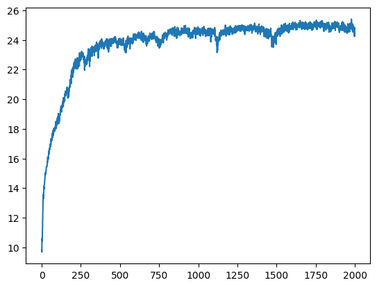
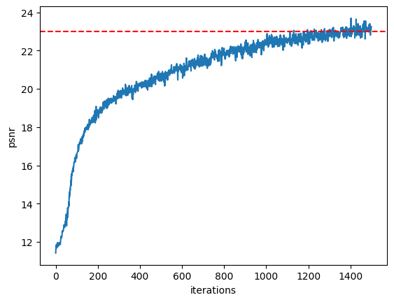
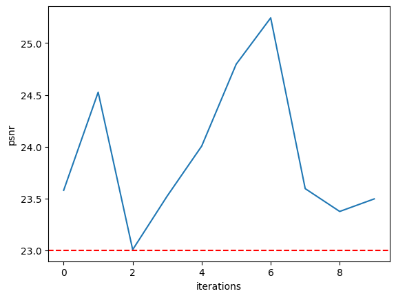
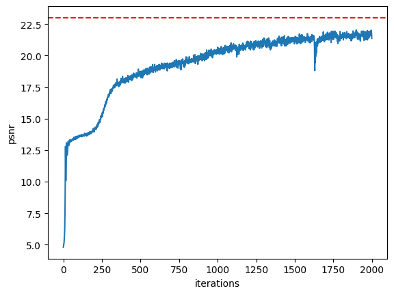
PSNR Curves
As you can see, the PSNR curve reaches above the goal of 23, and the average PSNR for the 10 images of the validation set with the trained model is 23.91.
Spherical Rendering (Novel Views)
Part 2.6 — NeRF Trained on My Own Captured Object
For this section, I trained a full Neural Radiance Field using the dataset captured in Part 0. This involved using my own calibrated images and camera poses, then training a NeRF model identical in structure to Part 2, with adjustments to near/far ranges and sampling strategy due to the much smaller physical scale of the scene.
Model Architecture & Training Setup
I used a custom NeRF architecture with skip connection, separate density/color branches, and independent positional encoding frequencies for 3D sample points and view directions.
Hyperparameter & Implementation Adjustments
- near = 0.2 and far = 0.5 (real-world scene was much smaller than Lego dataset)
- 64 samples per ray, jittered during training
- Positional encoding: Lx = 10 for positions, Lr = 4 for directions
- Adam optimizer: lr = 5e-4
These adjustments were essential to avoid the model sampling empty space and to keep rays bounded within the tight capture volume around the object.
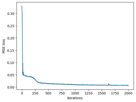
Training Loss Over Time
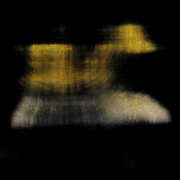
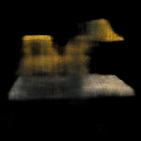
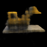
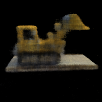
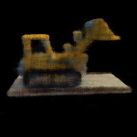
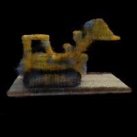
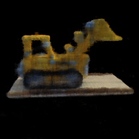
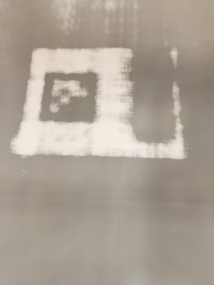
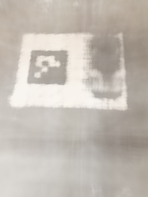
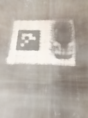
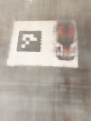
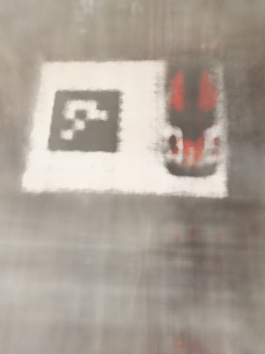
Intermediate Training Renders
Below are snapshots of the NeRF’s output at various stages of training. These demonstrate how density and color predictions refine over time.

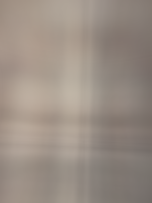
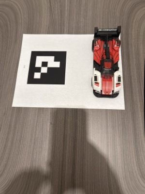
Reference Image
Novel-View Rendering (Final)
After training, I generated a 360° orbit animation by using the provided “look-at-origin” camera generation code, producing a smooth camera path around the object. Because my Aruco tag was so big, I pointed it towards a different corner rather than the origin corner. Thus, I had to change the logic for the roation function to rotate along a different world point. The final rendered GIF is shown below:
Conclusion
I implemented a complete Neural Radiance Field pipeline from scratch. From camera calibration and PnP, to neural fields, ray sampling, and full volumetric rendering, this project deepened my understanding of differentiable rendering and scene representation. THANKS FOR VIEWING MY PROJECT!!!